Stitching Photo Mosaics

Varun Bharadwaj - CS 180

Part A: Image Warping and Mosaics

Step 1: Taking Images

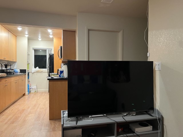
My Living Room
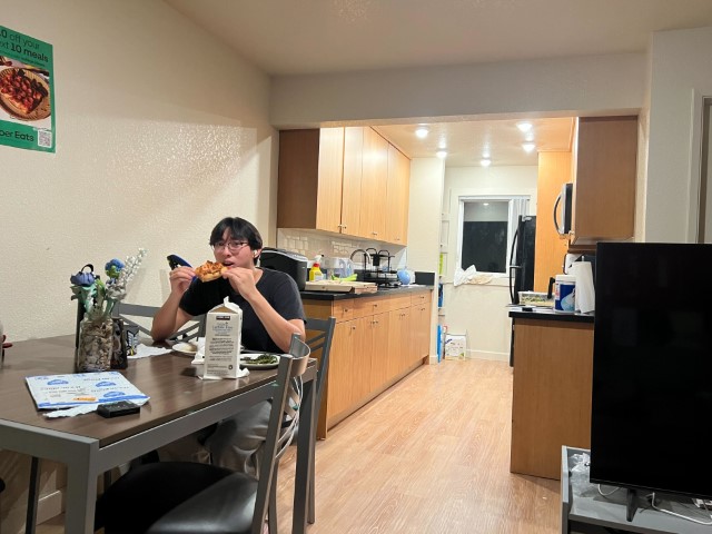
Image 1 of living Image 2 of living

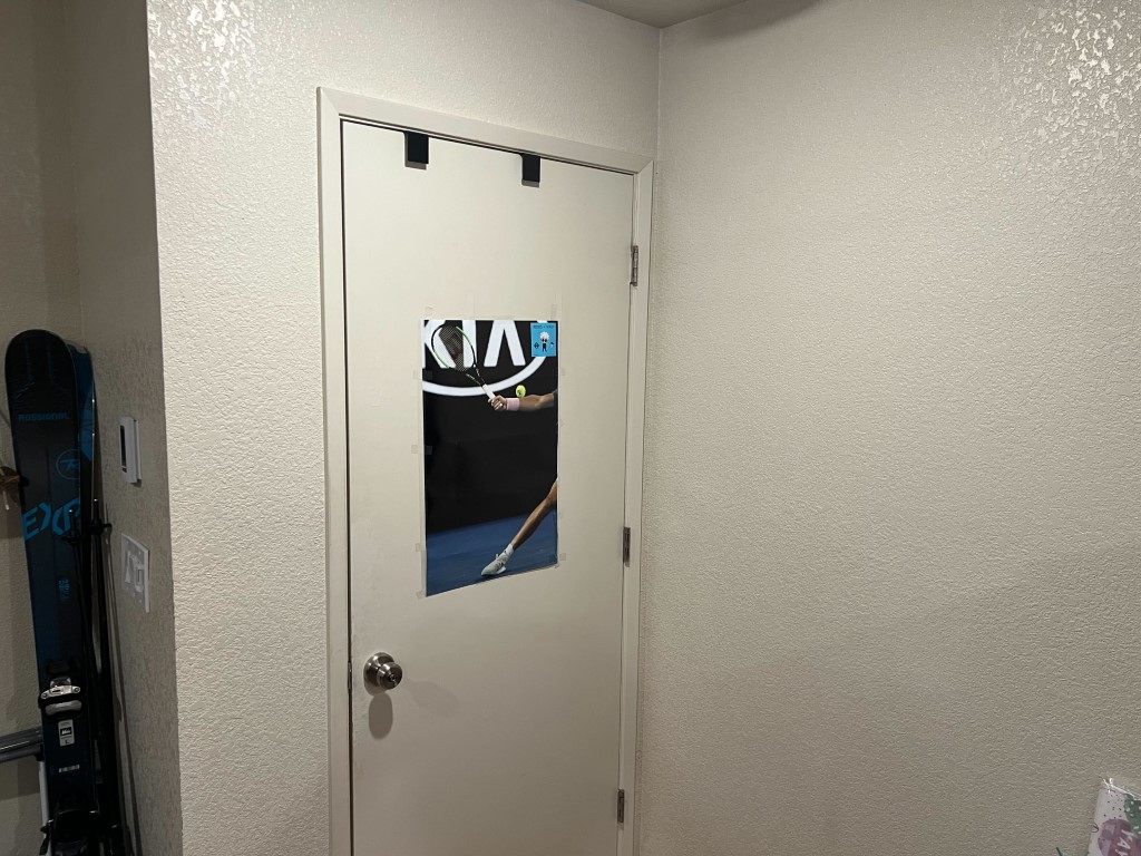
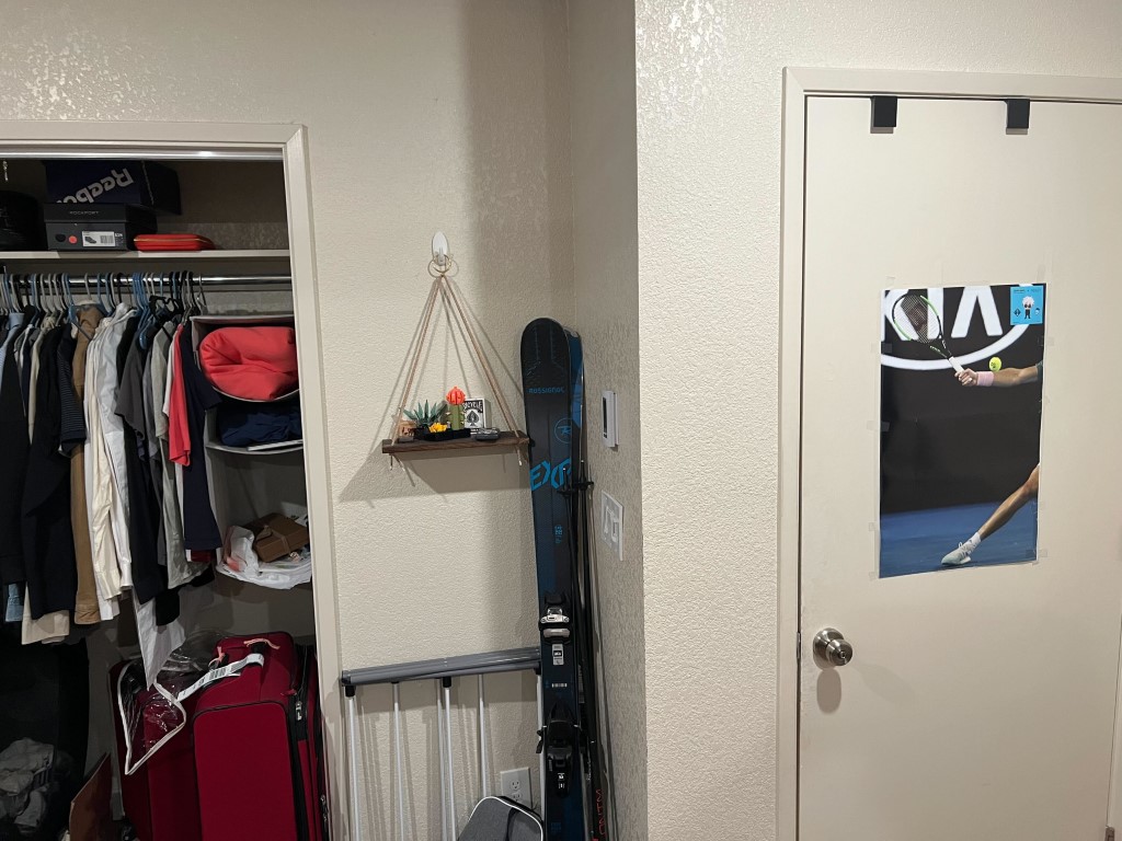
My Housemate's Bedroom

Image 1 of room Image 2 of room

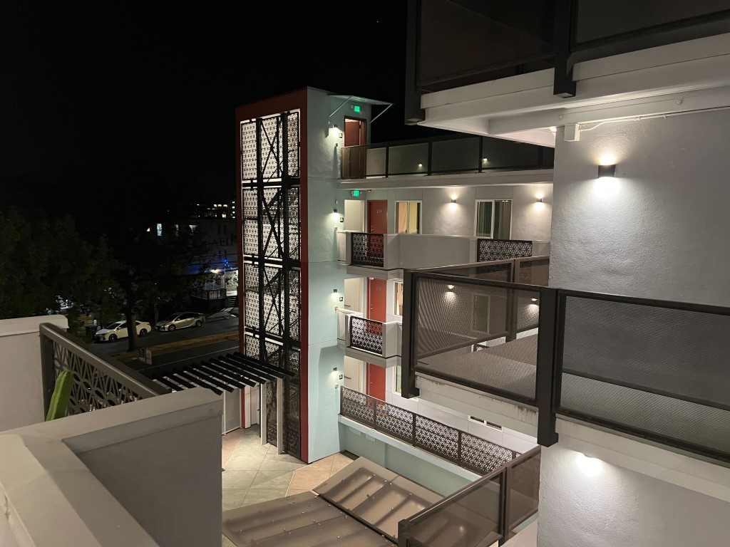
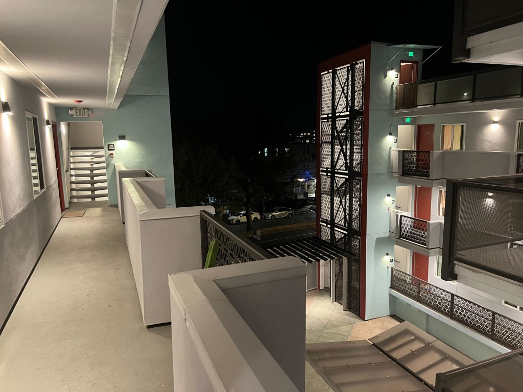
Outside my Apartment

Image 1 of outside Image 2 of outside

Step 2: Recovering Homographies

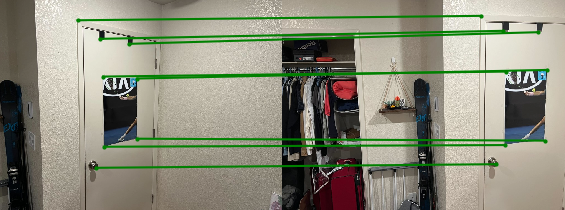
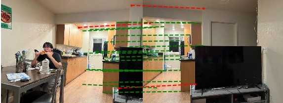
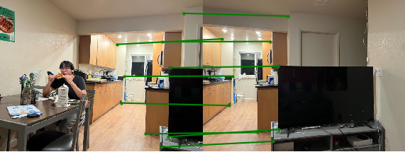
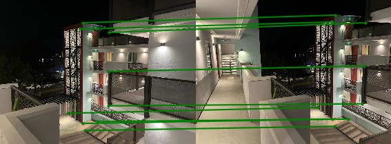
In order to get a projective mapping between the common features in the first image and the second image, we have to first find pairs of corresponding points. I do this by hand labelling matching corners in the images. I chose point first and second images. When labelling points that match in images, I tend to pick points at corners of recognazible features as they allow for accurate correspondences between images. As you can see in the examples I used features such as the corners of TVs, doorframes, walls, countertops, posters, and tables.
Description of image 1 for step 2 Description of image 1 for step 2
Description of image 1 for step 2

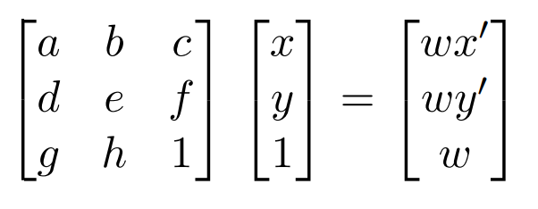
After getting pairs of points, we want to find a mapping that can morph points in the first image into their corresponding location in the second image. We want to find a projective transformation that solves the following systems of linear equations.
Description of image 1 for step 2

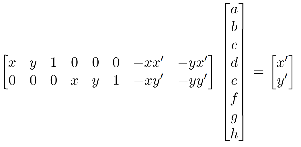
We can compute this H matrix by modifying this original equationt o get an alternate system of equations with the variables of H as the parameters.
Description of image 1 for step 2

We can then use the points that we have manually labelled as the values for x, y, x', and y' to create a solvable system of equations. However, due to noise in both the image capturing and correspondnece matching we need to find an approximate solution using Least Squares to apprximate a solution for the values of H.

Step 3: Warp the images

We will be using inverse warping in order to warp the images. To do this we first need to create a bounding box for the final warped image. I do this by using the homograph that we calculated in the previous part to map the corners of the original image to their new location in the warped image. After this, the process was similar to the inverse warping that we used in project 3. We use the homography that we calculated in the previous step in order to get a mapping for each pixel to its original location, and then used interpolation to get the specific color.

Step 4: Image Rectification

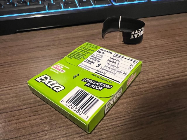
To test the code from part 3, I used image rectification to rectify rectangular objects. I did this by first taking a picture of a notebook and piece of gum on my desk. Since I didn't take a picture of these from directly above, they were not perfect rectangles in the original image.
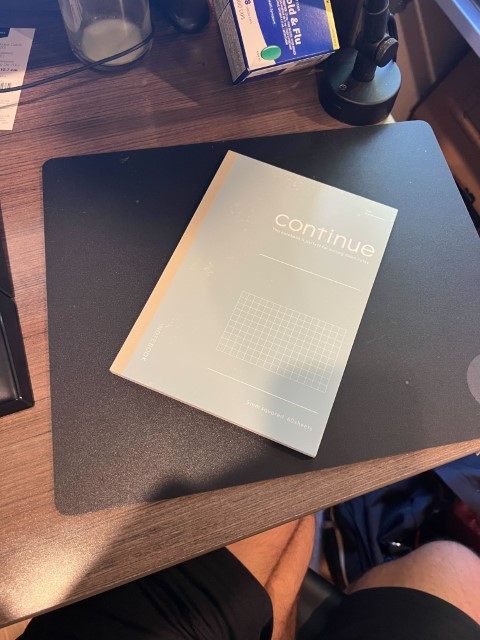
Description of image 1 for step 2 Description of image 1 for step 2

I then performed image rectification, which transformed these by morphing these rectangular objects onto a rectangle to orient it to be aligned with the edges of the image. Below we can see the results of the rectification of these images.
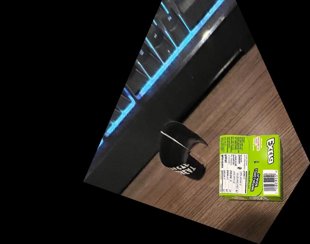
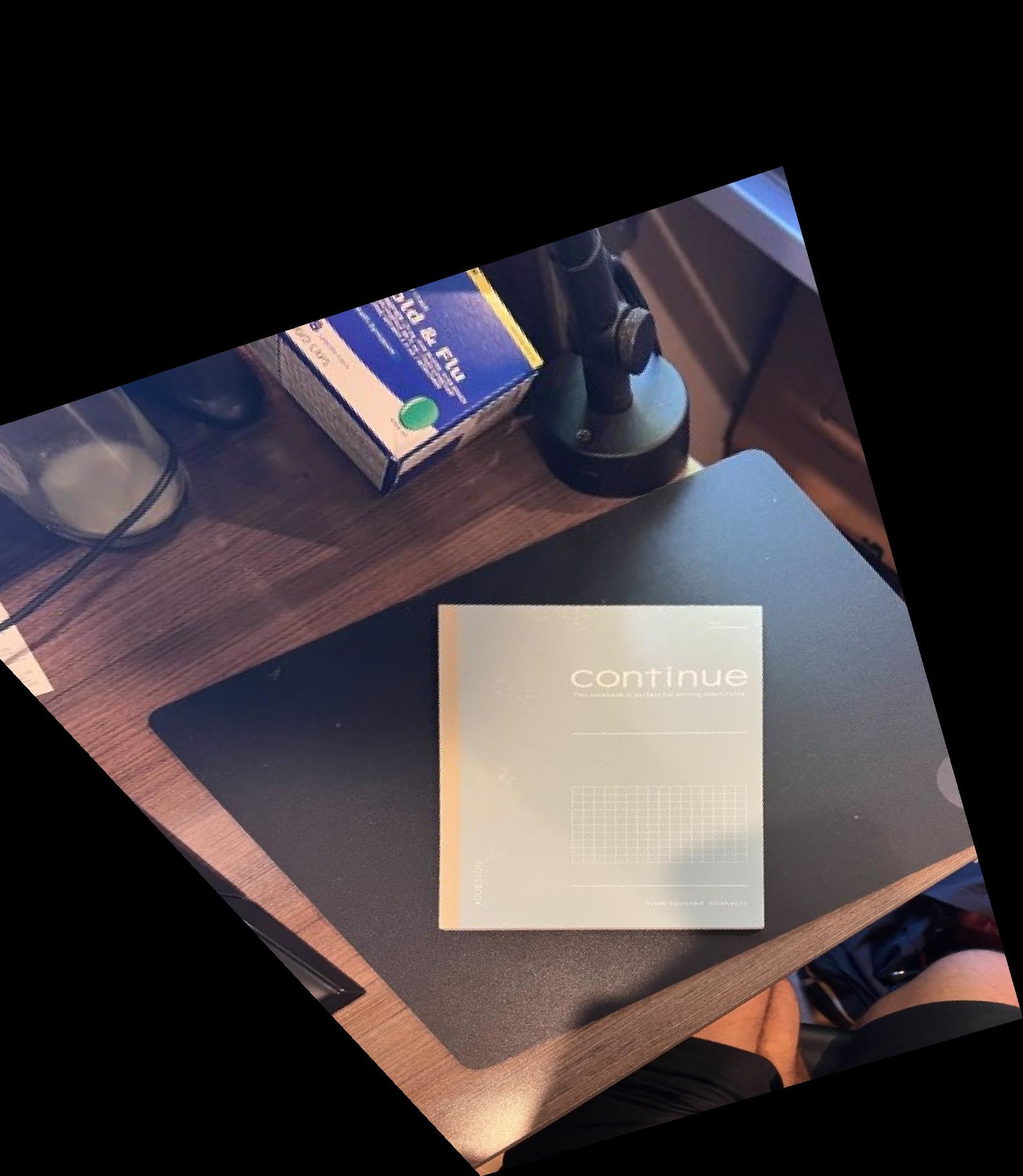
Description of image 1 for step 2 Description of image 1 for step 2

Step 5: Mosaics

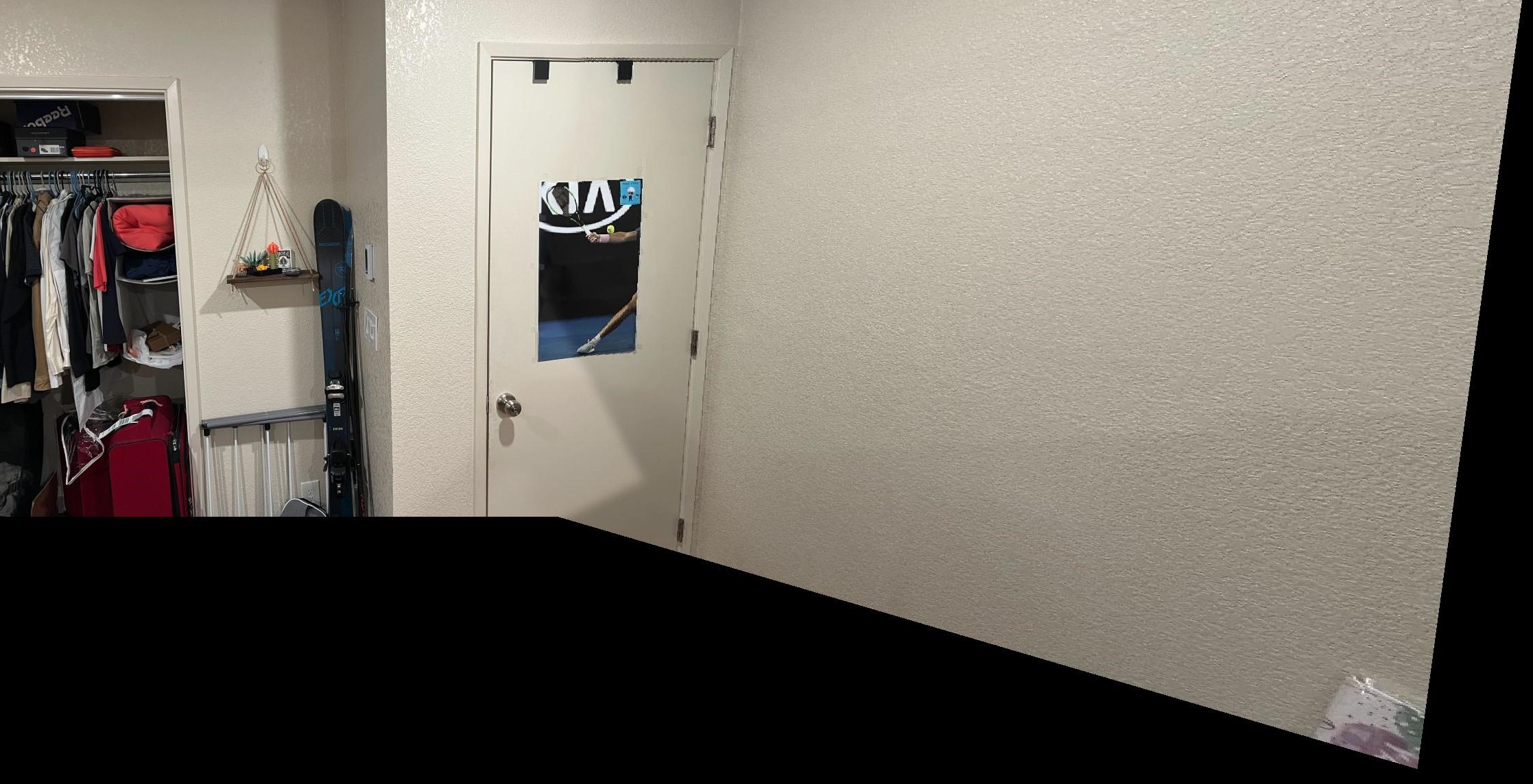
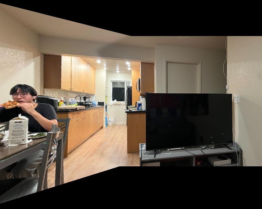
After warping the original image, we need to properly blend the 2 images together. Simply averaging the 2 images together will not work properly because small differences in lighting will become apparent, and there will be a clear boundary between the 2 images.
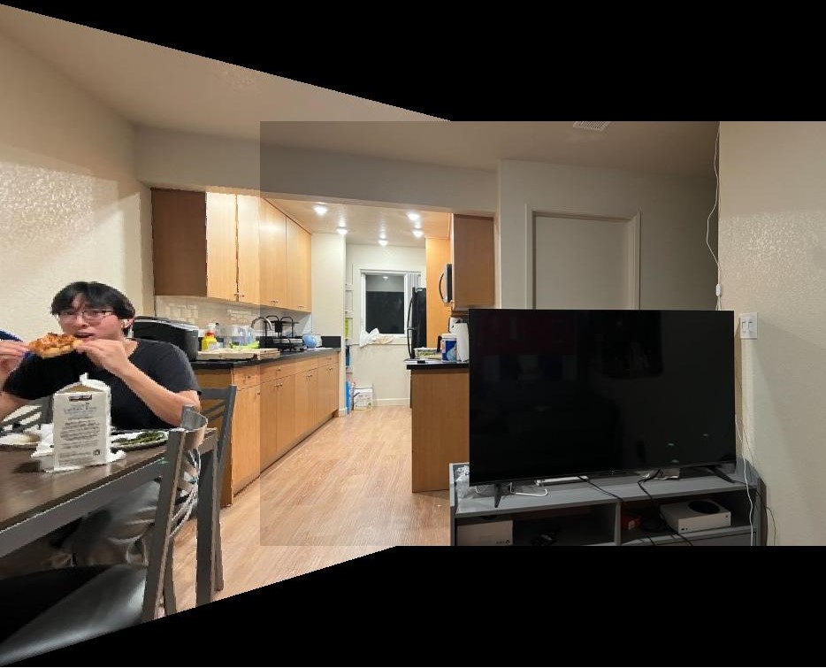
Description of image 1 for step 2

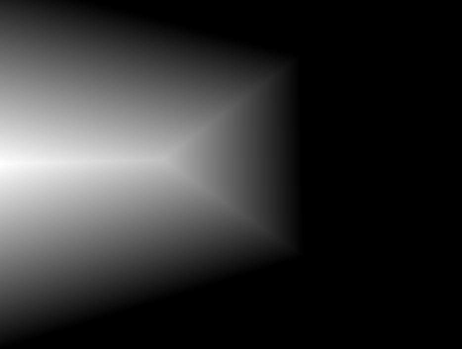
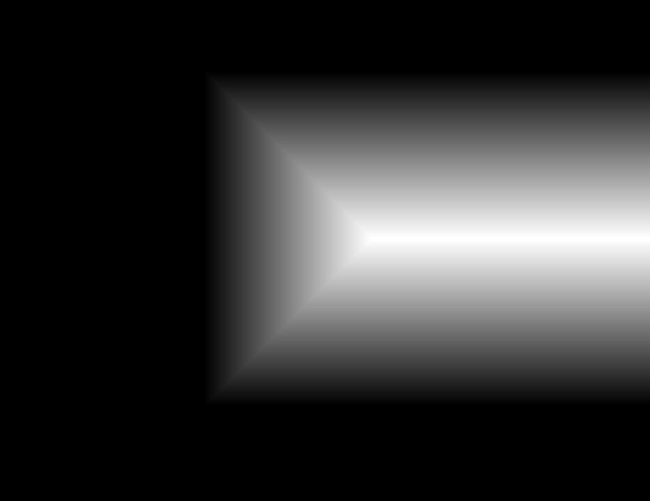
As you can see in the previous image, although the images are properly aligned doing a naive warp leaves a very clear border between the 2 images. To combat this, we instead do multi-resolution blending to remove this seam. To do this, we first need to create an alpha mask that tells the blending algorithm how much of each image to use at each pixel. We can do this by first, calculating a distance transform on the bounding box of each image. This gives the distance from each pixel in either image to the edge of it's bounding box. We can then run a pixel-wise comparison on these 2 bounding boxes in order to develop a larger mask that can be used to blend the 2 images.
Description of image 1 for step 2 Description of image 1 for step 2

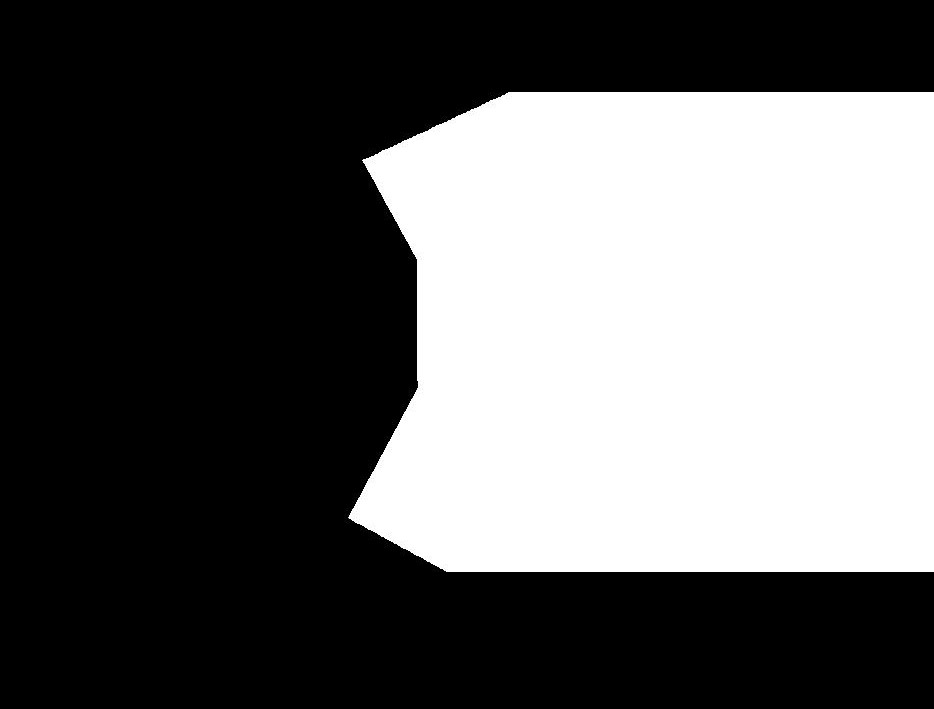
For each of these 2 distance transforms, if image 1's distance is greater, we will set the mask at that pixel to 0, and the opposite if image 2's distance is greater. Doing so gives us this final mask that we can use for 2-level multi-resolution blending.
Description of image 1 for step 2

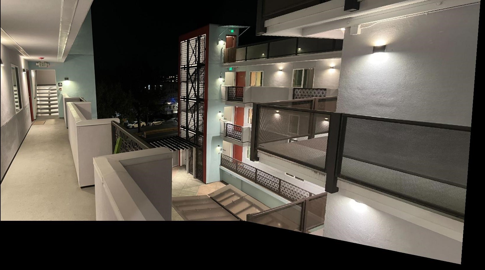
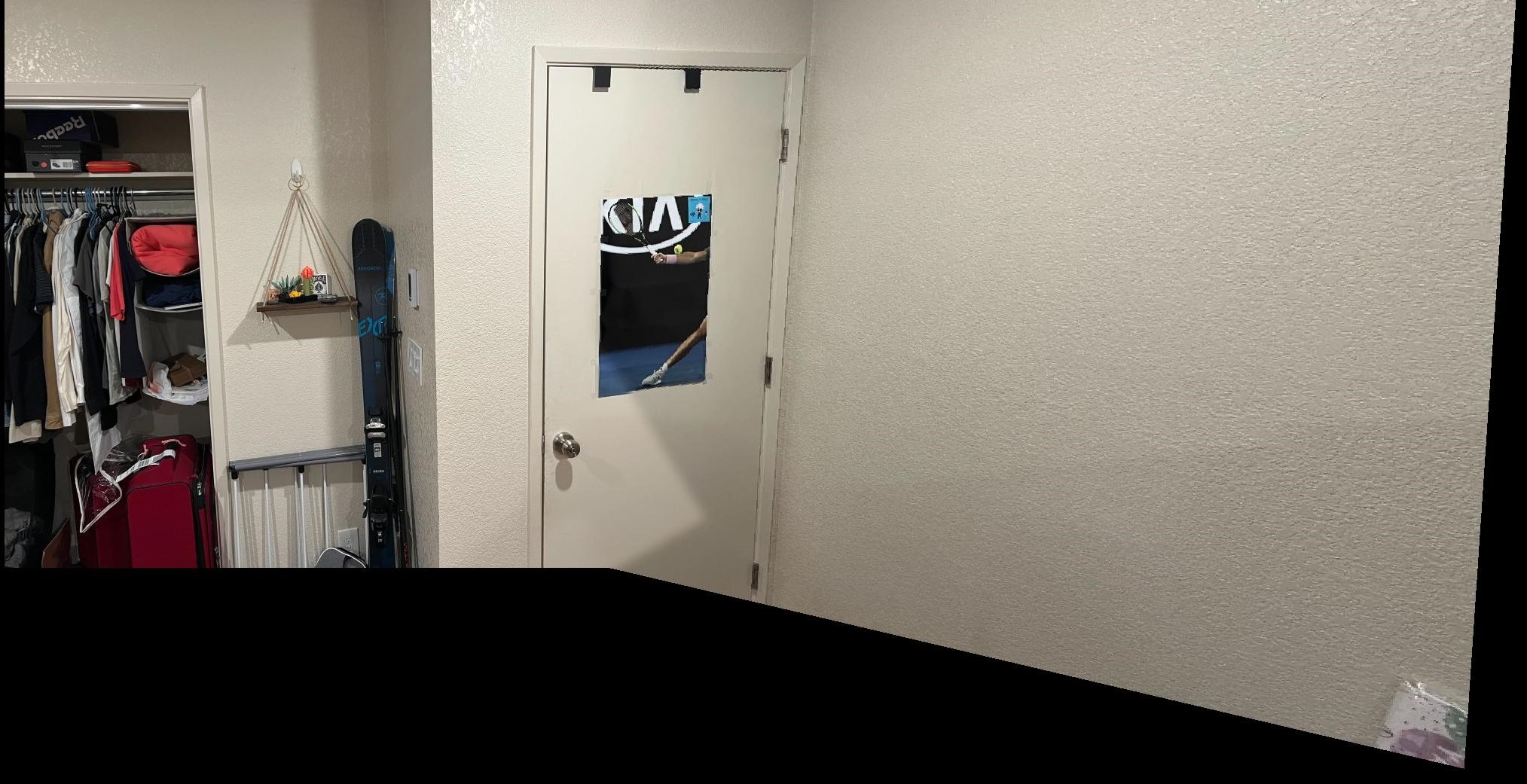
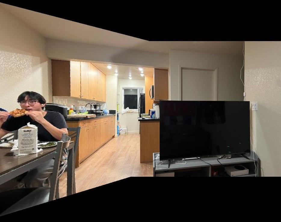
Finally we can use the multi-resolution blending that we implemented in project 2 to build the warped 1st image and second image using the mask we just created. Doing so gives us the following resoluts for the 3 images that I took in the first part of the project.
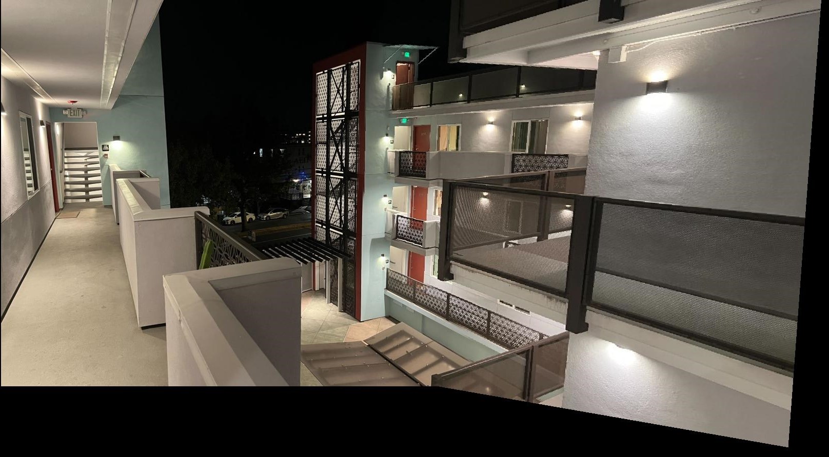
Description of image 1 for step 2
Description of image 1 for step 2 Description of image 1 for step 2

Part B: Feature Matching and Autostitching

Step 1: Corner Detection

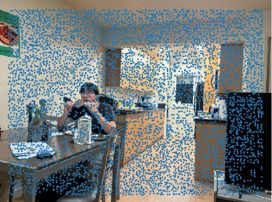
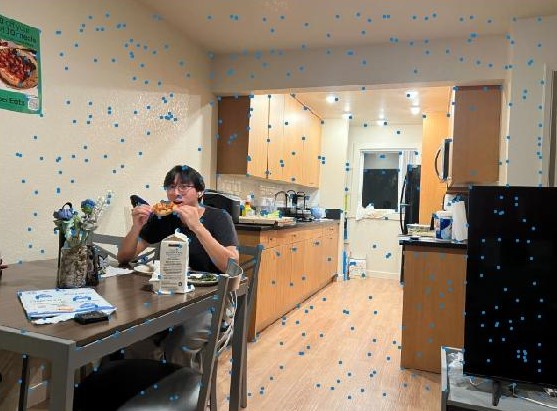
In order to generate a set of potential corners that can serve as features, we use a Harris point detector in order to generate potential corners of interest. The Harris corner detector generates over 6700 different corners as you can see below, so we must do additoinal processing in order to find the best features and points to match.

Description of image 1 for step 2

Here we can see the corners that the Harris point detector returned. There is a lot of noise due to it picking up corners such as the pepperoni on the Uber Eats poster, the small edges on the texture of the wall, and a bunch around my friend's hair. These are not all very helpful, so we need to find a way to select only the highest corners out of all of these.

Step 2: Adaptive Non-maximal Supression

To reduce the set of corners to look at we can do adaptive non maximal supression. This is an algorithm that given a set of possible corners, finds the highest quality corners. We want the corners to be spatially distributed over the image and to be strong. The way that this is done is by finding the largest radius r, such that there are 500 points that are all larger than all other points within r pixels of itself. This ensures that we are spatially distributing our points well and having strong corners.

Description of image 1 for step 2

Here we can see the corners that the ANMS point filtering returned. There is a lot of less noise, and this serves as a stronger smaller set to do feature matching on.

Step 3: Feature Extraction

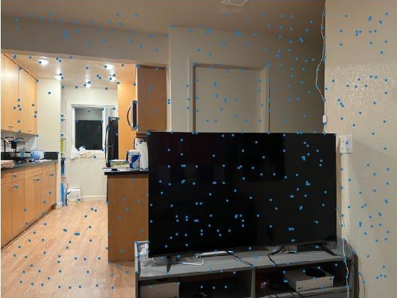
Now that we have 500 possible corners in 2 images, we can being working on trying to match features between the images. Below I have attached the 2 images and their ANMS supressed corners.

Description of image 1 for step 2 Description of image 1 for step 2

For each point in the corner set for both images we can extract the features by taking the 40x40 pixel area around the corner, resize it down to an 8x8 feature and then normalize the feature by subtracting the mean and dividing the standard deviation. This for each corner gives us a comparable feature that we can use to find matches between images. Below I have put 5 features for corners in the first image.

Description of image 1 for step 2 Description of image 1 for step 2 Description of image 1 for step 2 Description of image 1 for step 2 Description of image 1 for step 2

Step 4: Feature Extraction

After getting the features from the feature extractor, the next step is to match corresponding features in both images. The way that this is done is by finding the feature in the corresponding image that has the closest l2 distance from the current feature. A trick that we can do in order to further filter out features that are not in the other image and noisy outliers from the real corresponding corners is by using Lowe's thresholding. What we do here is we add an additional constraint that for in order for a feature to be matching, we also require that the l2 distance between the closest corresponding feature is at least twice as big as the l2 distance to the 2nd closest corresponding feature. What this does is that it ensures that feature matches are more likely to be real features as oppossed to coincidences and noise. Below I have put some of the matched features

Matching Feature 1:

Description of image 1 for step 2 Description of image 1 for step 2

Matching Feature 2:

Description of image 1 for step 2 Description of image 1 for step 2

Matching Feature 3:

Description of image 1 for step 2 Description of image 1 for step 2

Matching Feature 4:

Description of image 1 for step 2 Description of image 1 for step 2

Matching Feature 5:

Description of image 1 for step 2 Description of image 1 for step 2

Step 5: Ransac

Finally, we would like to calculate a homography from these points. However, it isn't the best to use all of the points that we have since outliers will have filtered through and they can have a large impact on the final homography. Instead we can use RANSAC in order to find a choice of 4 points that best translates the most correspondences that we have found. This can be done by randomly sampling 4 points in our set of correspondences, calculating the homography between them, calculating the number of other points that match this homogrpahy (within some error). Finally, we simply pick the best homography after repeating this process 5000 times.

Description of image 1 for step 2

Here we can see the inliers that RANSAC was able to calculate.

Results

We can use these calculated homographies in order to perform a fully automatic mosaic on images. Here are the results from the images I took in the beggining

Description of image 1 for step 2
Description of image 1 for step 2 Description of image 1 for step 2